How to Freeze Top Row and First Column in Excel

When you work with wide and tall worksheets it helps to keep headers and key identifiers visible while you scroll. Here is a step-by-step guides.

Step-by-step (Windows and Mac Excel)

1. Click cell B2. This tells Excel you want everything above and to the left of that cell frozen.
2. Go to the View tab on the ribbon.
3. Click Freeze Panes.
4. Choose Freeze Panes from the dropdown.

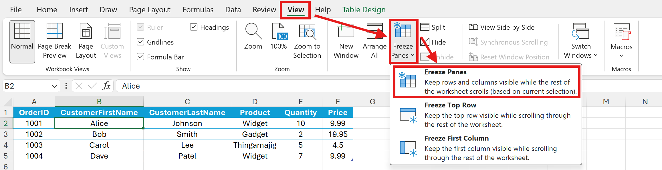
After that, row 1 will remain fixed at the top and column A will remain fixed at the left while you scroll the worksheet.

Quick variations

• To freeze only the top row use View > Freeze Panes > Freeze Top Row.
• To freeze only the first column use View > Freeze Panes > Freeze First Column.

How to unfreeze panes

• Go to View > Freeze Panes > Freeze Panes. This returns the sheet to normal scrolling.